Part 3 New York Genome Center

Whole genome sequencing and analysis was done at the New York Genome Center by the production, Erlich, and Pickrell labs.

1) Data Preparation

Alignment was performed using BWA [1] and variant calling with GATK HaplotypeCaller [2] as part of the standard NYGC WGS pipeline.

By definition, VCF files contain sites called different from the reference genome. In order to upload the output to DNA.Land for ancestry inference and relative matching, we need to also include sites where both alleles match the reference genome.

The gVCF is a compressed version of a standard VCF, in which contiguous, non-variant regions are compressed into single records. Homozygous reference blocks were broken using gvcftools “break blocks” [3] and only sites in 23andMe genotyping were kept. This file was then uploaded to DNA.Land.

Quality Control

Before doing any meaningful analysis, we need to make sure the sequencing results match certain quality control expectations. This includes assessing mean coverage across the genome (ie. the average number of times each base is sequenced), the transition/transversion ratio (Ti/Tv), the ratio of nonsynonymous/synonymous substitutions, heterozygous to homozygous variants, and verifying the sex of the individual (homozygosity across X chromosome markers).

Heterozygosity is a measure of inbreeding as well as DNA sample quality. Observed and expected autosomal homozygous genotype counts were computed for each sample using plink2 [6]. Mean heterozygosity is simply the difference of non-missing genotypes and the observed number of homozygous genotypes divided by the number of non-missing genotypes. Too little heterozygosity can be indicative of inbreeding and too much may suggest sequencing sample contamination.

These metrics were calculated using coverageBed [4], VCFtools [5], and plink2 [6]. Finally, we used SnpEff [7] to annotate and predict effects of we annotate the variants in the resulting VCF.

Some QC metrics for Carl’s whole genome:

Total SNVs	5176100
Total known SNVs	4707403
Total novel SNVs	468697
Mean coverage	35.347681
Ti/Tv	1.97
Het/Hom	1.85

2) Ancestry Analysis

Principal Component Analysis

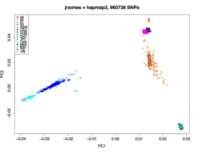
We filtered Carl’s VCF along with 3 Ashkenazi samples, and converted these files to plink format (http://pngu.mgh.harvard.edu/~purcell/plink/data.shtml), a compressed version of the whole genome data that allows for faster analysis. We then merged this data with data from the 1000 Genomes Project (phase 3) [8], which includes whole genome sequencing of 1397 samples from 11 populations (for population details, see http://www.1000genomes.org/faq/which-populations-are-part-your-study/).

We pruned SNPs so that markers are in approximate linkage equilibrium and performed PCA using plink2 [6]. This generates Eigen vectors, which are basically new coordinates (principal components) that can be plotted to display high-dimensional data in 2D. The first principal component is the direction of the largest variance in the data and the second is the direction in which the largest part of the remaining variance occurs and so on. PCA can reduce a complex dataset to see if there’s any hidden structure, such as population stratification.

PCA HapMap Phase 3 and 4 AJ samples (Carl=59) (pdf)

jn_hapmap3_plink_pca

We then performed PCA after incorporating additional genotype data from 471 Ashkenazi Jewish individuals [17]. After filtering and QC, 33260 markers with a genotyping rate of >0.99 in 923 males and 949 females were used in the analysis. If we plot the second and third PCs (below), we see that Carl falls between the European populations (“TSI” and “CEU”) and the Ashkenazi (“AJ”) samples (yellow).

PCA HapMap Phase 3, 471 AJ, and our 4 AJ samples (Carl=59) (pdf)

jn_hapmap_bray_pca_2v3

Mitochondria Haplogroup

Mitochondrial haplogroup (h1ag1) was determined by tracing the lineage of mitochondrial mutations in the final VCF to mtDNA tree Build 17 from Phylotree [10] (mt_mutations.txt).

G3010A, H1

A6272G, H1ag1

G14869A, H1ag

Y Halpogroup

Y haplogroup was determined by calling Y-STRs using lobSTR [11]. Alleles for each marker were determined by dividing the lobSTR allele by the STR period and summing this value and the reference allele. The results (59.ftdna.markers) were entered into the Haplogroup Predictor 27-Haplogroup Program [12] (FTDNA order, Northwest Europe), which predicted haplogroup E1b1 with the highest probability.

We used an orthogonal method (AMY-tree v2.0) [13] that determines haplogroup using Y chromosome SNPs. The same result (E1b1b1c1) was obtained by all analysis methods.

III. Global Ancestry

Ancestry analysis was performed using the Pickrell Lab’s ancestry v.0.01 inference algorithm [14]. This approach uses a reference set of labeled individuals to assign the individual to these populations, which have distinct per-locus allele frequencies.

Samtools mpileup [15] was used to convert bam files to a summary of base calls of aligned reads, including SNPs listed in the reference panel for input to the ancestry program, resulting in a total of 1,324,635 sites.

Global Ancestry Results:

ASHKENAZI	0.49611
ITALY-BALKANS	0.0768259
N EUROPE	0.349107
SW EUROPE	0.0701873 Local Ancestry

cz_ancestry

Local Ancestry:

To refine the continental ancestry analysis, we inferred local ancestry using RFMix [16]. Carl’s whole genome was first merged and phased together with 3 Ashkenazi whole genome samples and 1798 samples from the HGDP reference [9].

Only biallelic SNPs also found in the reference data were included from Carl’s VCF, which was then converted to plink format and merged with the HGDP reference data. Prior to phasing, individuals or sites with more than 5% missing genotypes and failing strand alignment were excluded. Monomorphic or singleton markers were also removed, as they are not informative for phasing.

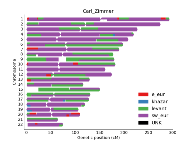
In order to proceed with the RFMix analysis, the admixed samples (Carl’s genome and 3 Ashkenazi Jewish individuals) were separated from the phased output (‘haps’ files). The reference population files were also edited to include 4 different population classes against which to compare the 4 admixed samples: Levant (Druze, Palestinian), SW Europe (French, Italian), E Europe (Russian), and Khazar (Adygei). We ran RFMix with 2 EM iterations, minimum node size 5 (recommended if reference sample sizes are skewed > 2:1 or is using EM), assumed 50 generations since admixture, and a window of 1 cM. We chose a larger window to include more SNPs since only ~300,000 overlap between our 4 admixed (mostly Ashkenazi) and reference samples.

After running RFMix, we collapsed the output into bed files and generated the below karyogram plots, including 1 example from each population used in the analysis.

carl_zimmer

Resources:

BWA: http://bio-bwa.sourceforge.net/

GATK: https://www.broadinstitute.org/gatk/

gvcftools: https://sites.google.com/site/gvcftools/home/

bedtools: bedtools.readthedocs.io/en/latest/index.html

VCFtools: http://vcftools.sourceforge.net/

plink2: https://www.cog-genomics.org/plink2/

snpEff: snpeff.sourceforge.net

1000 Genomes: http://www.1000genomes.org/data

HGDP: http://genetics.med.harvard.edu/reichlab/Reich_Lab/Datasets.html

PhyloTree: van Oven M, Kayser M. 2009. Updated comprehensive phylogenetic tree of global human mitochondrial DNA variation. Hum Mutat30(2):E386-E394. http://www.phylotree.org.