Part 3 Mason lab

Genome analysis from the Mason Lab, Weill Cornell Medicine (WCM)

(See also these slides for an overall report)

I. Ancestry

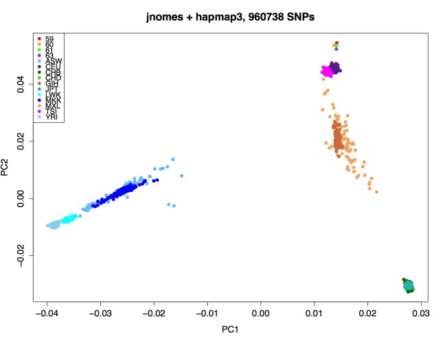
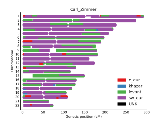
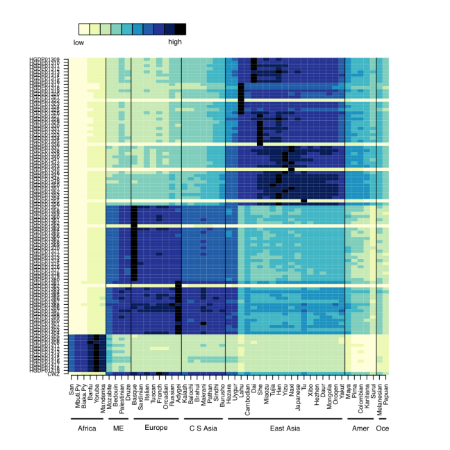
We first confirmed that CZ was indeed genetically male, based on the X-chromosome’s Loss of Heterozygosity (LOH), and this indeed was true (>98% homozygous SNV calls). Next, we wanted to look at the ancestry of CZ using Ancestry Mapper, a tool that allows you to calculate the genetic distance of a person’s genome relative to 51 reference populations, using over 1,000 individuals from the Human Genome Diversity Project. Interestingly, we also used this same algorithm to map the DNA left on subway surfaces with the neighborhood’s U.S. Census data (Black, White, Asian, Hispanic) and showed that neighborhoods’ DNA that often matched the Census data (Afshinnekoo et al., 2015). But, for CZ (bottom row, Figure 1), we found him closest to the French, Italian, and Basque reference populations, but also with similarity to European and Middle Eastern ancestry.

Figure 1- Predicted ancestry of CZ genome. Genetic similarities are plotted for a large set of reference populations (x-axis) from different regions of the world, including Africa, Middle East, Europe, Central South Asia, East Asia, Americas, and Oceania. CZ’s genome is at the bottom.

 subjectz_ancestrymapper_plot_inset

References :
Afshinnekoo E, Meydan C, Chowdhury S, Jaroudi D, et al. Mason CE. “Geospatial Resolution of Human and Bacterial Diversity from City-scale Metagenomics.” Cell Systems. 2015 Jul 29;1(1):72-87. PMC4651444.

Magalhães TR, Casey JP, Conroy J, Regan R, Fitzpatrick DJ, et al. (2012) HGDP and HapMap Analysis by Ancestry Mapper Reveals Local and Global Population Relationships. PLoS ONE 7(11): e49438.


II. QIAGEN’s Ingenuity Variant Analysis

Ingenuity Variant Analysis is a widely-used service used to analyze genomes by prioritizing variants through a series of cascading filters. CZ’s variants were ranked with the highest prioritized risk, based on their confidence, population frequencies, predictions of being deleterious, and comparison to known cancer drivers. At the end, these variants were associated with Epithelial and Head and Neck tumors (Figure 2).

Figure 2: Summary of Ingenuity’s Variant Interpretation of CZ’s genome. Filter cascades (left) show the removal of common and non-disease related variants, leaving a subset of 177 genes with 541 mutations that are related to cancer risk. The top-ranking cancers are epithelial and head and neck cancers.

subjectz_ingenuity_all_filters


III. Omicia and ClinVar for Clinical interpretation of risk and protective alleles (SNVs):

We next annotated variants using SnpEff software to identify variants in protein coding genes and assess impacts of variants on the protein product [1]. We further annotated these variants using the ClinVar database of pathogenic and non-pathogenic variants submitted through clinical channels on dbSNP and updated weekly; the version of the vcf format clinvar file used was from 03/02/2016 [2]. After filtering for quality and coverage (minimum quality score of 30 and minimum read depth of 10), we used these annotations to identify “high priority” variants, defining “high priority” as variants with moderate to high impact on protein sequence according to SnpEff and also present in the clinvar and OMIM (Online Mendelian Inheritance in Man) databases.

This identified 3,143 SNVs, of which 41 were marked by ClinVar as pathogenic and 5/41 SNVs as uncommon. These SNVs are in TERT, PRSS1 (2 SNVs), SAA1, and MEFV. Cross-referencing these SNVs with Omicia’s Opal Clinical software revealed that variants in MEFV lead to familial Mediterranean fever, but follow a recessive inheritance pattern, and since the variant identified was heterozygous, this SNV is thought to not have a phenotypic effect. The TERT variant (p.His412Tyr) is linked to shorter telomere lengths. PRSS1 variants are associated with hereditary pancreatitis, and the SAA1 variant (p.Ala70Val) may increase risk of reactive systemic amyloidosis (AA-amyloidosis) which is a rare complication of common chronic inflammatory diseases such as rheumatoid arthritis [3].

However, there were some mutations with good news. Specifically, mutations in C2 and CFB conferred a protection against age-related macular degeneration. Also, three mutations in IL23R revealed a lower risk of inflammatory bowel disease (IBD) and psoriasis (autoimmune). Moreover, protection against type II diabetes (MTTP), myocardial infarction and venus thrombosis (F13A1), and coronary heart disase (ABCA1) were all present. These indicate a genetic catalog of alleles with lower risk than the general population.


[1]      P. Cingolani, A. Platts, L. L. Wang, M. Coon, T. Nguyen, L. Wang, S. J. Land, X. Lu, and D. M. Ruden, “A program for annotating and predicting the effects of single nucleotide polymorphisms, SnpEff: SNPs in the genome of Drosophila melanogaster strain w1118; iso-2; iso-3.,” Fly (Austin)., vol. 6, no. 2, pp. 80–92, Jan. .

[2]      M. J. Landrum, J. M. Lee, G. R. Riley, W. Jang, W. S. Rubinstein, D. M. Church, and D. R. Maglott, “ClinVar: public archive of relationships among sequence variation and human phenotype.,” Nucleic Acids Res., vol. 42, no. Database issue, pp. D980–5, Jan. 2014.

[3]      S. Baba, S. A. Masago, T. Takahashi, T. Kasama, H. Sugimura, S. Tsugane, Y. Tsutsui, and H. Shirasawa, “A novel allelic variant of serum amyloid A, SAA1 gamma: genomic evidence, evolution, frequency, and implication as a risk factor for reactive systemic AA-amyloidosis.,” Hum. Mol. Genet., vol. 4, no. 6, pp. 1083–7, Jun. 1995.

IV. Non-coding mutated genes

Beyond the protein-coding genes, there are many regulatory and non-coding genes across the genome that also can mediate disease or phenotypes. We scanned CZ’s genome for non-reference alleles and then intersected these variants with ENCODE regions and other regulatory regions such as VISTA enhancers. The transcription-factor binding sites with the most mutations were:

  • STAT4 (Signal Transducer And Activator Of Transcription)
  • AP1 (Activator Protein 1)
  • EGR1 (nerve growth)
  • AP2GAMMA1 (neural crest)
  • GATA1 (hematopoietic TF)

There were also some VISTA enhancers (http://enhancer.lbl.gov) with an enrichment in mutations relative to the general population, and this included:

1) element 2082

dorsal root ganglion, trigeminal V (ganglion, cranial)

2) element 2084

other

3) element 1760

heart

4) element 1886

heart

5) element 1385

hindbrain (rhombencephalon), midbrain (mesencephalon)

6) element 1391

midbrain (mesencephalon), forebrain

However, CZ’s body is already fully developed, so clearly these mutations did not prevent him from forming a complete midbrain, heart, or hindbrain. Which is good news, especially for CZ.

(See slides for more details)

V. Transposable Element Insertions (TEIs)

We next used a computational tool called Jitterbug (https://github.com/elzbth/jitterbug) to scan for transposable element insertions (TEIs) that have inserted into CZ’s genome. We found 452 TEIs present in CZ’s genome, but all of these are also predicted from normal controls in the Pan-Cancer analysis of Whole Genomes (PCAWG) normal samples, n=64 controls), and thus they represent normal genetic variation.

Interestingly, 4 of these TEIs (Alus) are in introns, of the following genes:

MIR7641-2, RBM6, BRWD1, ENY2.

And 11 TEIs are in common with Genome in a Bottle GIAB) trio (son, father, mother):

HG002: 6, HG003: 5, HG004: 9

(See slides for more details)


Advertisement

Part 3 Feschotte lab

Aurélie Kapusta & Cédric Feschotte, University of Utah School of Medicine

I. Building the known loci coordinates file from references [1,2]

We used the data from references [1,2] and labeled them (“no_ref”, “ref_variable” and “ref_polym” based on ref. [2] Dataset_S03, ] and “MacFarlane” for the loci listed in ref. [1]), see the file HERVKloci.bed

The coordinates in that file correspond to the empty site for the “no_ref” ones as well as the locus 19p12c [1] (see case 1 from SubjectZ_HERVK_schema.pptx), and otherwise to the 5’ end junction, meaning 5’ flanking DNA + HERV-K LTR DNA sequences (see case 2 from SubjectZ_HERVK_schema.pptx). Exact coordinates can be found in the file HERVKloci.bed, and more details in the excel file

The bam file has numbers without the label chr for the chromosome numbers, replace:

sed –i ‘s/chr//’ HERVKloci.bed > HERVKloci.bed


II. Intersect with the coordinates of the genomic reads of SubjectZ

We used bedtools v2.25.0 [3].

Just to be safe, sort the loci file:

sortBed -i HERVKloci.bed > HERVKloci.sorted.bed

First, to avoid some errors (“…has inconsistent naming convention for record”), we converted the bam file to bed file:

bamToBed -i PG0004515-BLD.final.bam > PG0004515-BLD.final.bed &

Additionally, to avoid some kill errors, we extracted subsets of reads prior to intersection:

nohup grep “^X” PG0004515-BLD.final.bed > PG0004515-BLD.final.chrX.bed &

nohup grep “^Y” PG0004515-BLD.final.bed > PG0004515-BLD.final.chrY.bed &

nohup grep “^1” PG0004515-BLD.final.bed | grep -v -E “^1[0-9]” > PG0004515-BLD.final.chr1.bed &

nohup grep “^2” PG0004515-BLD.final.bed | grep -v -E “^2[0-9]” > PG0004515-BLD.final.chr2.bed &

nohup grep -E “^1[0-4]” PG0004515-BLD.final.bed > PG0004515-BLD.final.chr10-14.bed &

nohup grep -E “^1[5-9]” PG0004515-BLD.final.bed > PG0004515-BLD.final.chr15-19.bed &

nohup grep -E “^2[0-2]” PG0004515-BLD.final.bed > PG0004515-BLD.final.chr20-22.bed &

nohup grep -E “^[3-4]” PG0004515-BLD.final.bed > PG0004515-BLD.final.chr3-4.bed &

nohup grep -E “^[5-6]” PG0004515-BLD.final.bed > PG0004515-BLD.final.chr5-6.bed &

nohup grep -E “^[7-9]” PG0004515-BLD.final.bed > PG0004515-BLD.final.chr7-9.bed &


Then we ran the intersections:

nohup intersectBed -a HERVKloci.sorted.bed -b PG0004515-BLD.final.chrX.bed -wo > HERVKloci.CZbed.chrX.bed &

nohup intersectBed -a HERVKloci.sorted.bed -b PG0004515-BLD.final.chrY.bed -wo > HERVKloci.CZbed.chrY.bed &

nohup intersectBed -a HERVKloci.sorted.bed -b PG0004515-BLD.final.chr1.bed -wo > HERVKloci.CZbed.chr1.bed &

nohup intersectBed -a HERVKloci.sorted.bed -b PG0004515-BLD.final.chr2.bed -wo > HERVKloci.CZbed.chr2.bed &

nohup intersectBed -a HERVKloci.sorted.bed -b PG0004515-BLD.final.chr10-14.bed -wo > HERVKloci.CZbed.chr10-14.bed &

nohup intersectBed -a HERVKloci.sorted.bed -b PG0004515-BLD.final.chr15-19.bed -wo > HERVKloci.CZbed.chr15-19.bed &

nohup intersectBed -a HERVKloci.sorted.bed -b PG0004515-BLD.final.chr20-22.bed -wo > HERVKloci.CZbed.chr20-22.bed &

nohup intersectBed -a HERVKloci.sorted.bed -b PG0004515-BLD.final.chr3-4.bed -wo > HERVKloci.CZbed.chr3-4.bed &

nohup intersectBed -a HERVKloci.sorted.bed -b PG0004515-BLD.final.chr7-9.bed -wo > HERVKloci.CZbed.chr7-9.bed &

nohup intersectBed -a HERVKloci.sorted.bed -b PG0004515-BLD.final.chr5-6.bed -wo > HERVKloci.CZbed.chr5-6.bed &


III. Visualize the genomic reads of SubjectZ in the UCSC genome browser

Thanks: Edward B. Chuong

We used bedtools v2.25.0 [3] and samtools v.1-3 [4]

To visualize the reads in UCSC genome browser, we needed to add the chromosome numbers in the bam file:

http://seqanswers.com/forums/showthread.php?t=22504

nohup samtools view -h PG0004515-BLD.final.bam | awk ‘BEGIN{FS=OFS=”\t”} (/^@/ && !/@SQ/){print $0} $2~/^SN:[1-9]|^SN:X|^SN:Y|^SN:MT/{print $0}  $3~/^[1-9]|X|Y|MT/{$3=”chr”$3; print $0} ‘ | sed ‘s/SN:/SN:chr/g’ | sed ‘s/chrMT/chrM/g’ | samtools view -bS – > PG0004515-BLD.final.chr.bam &


Generate the associated .bai:

nohup samtools index PG0004515-BLD.final.chr.bam > PG0004515-BLD.final.chr.bam.bai.log &


Generate the required files:

nohup bedtools genomecov -bg -ibam PG0004515-BLD.final.chr.bam -g hg19.chrom.sizes > PG0004515-BLD.final.chr.bdg &

wget http://hgdownload.cse.ucsc.edu/admin/exe/linux.x86_64/bedGraphToBigWig

nohup ./bedGraphToBigWig PG0004515-BLD.final.chr.bdg hg19.chrom.sizes PG0004515-BLD.final.chr.bw > PG0004515-BLD.final.chr.bw.log &


Then these files were uploaded by Ed Chuong to his own Amazon account and loaded as a track in the UCSC genome browser. This allowed us to check specific loci and take the screen shots showed the associated file in results (SubjectZ_HERV-K_screenshots.pptx).


IV. Check the loci in the HuRef (Craig Venter’s genome) assembly

We used blast 2.2.29+ [5]

a. Loci from ref [1]

Fasta files were downloaded from:

ftp://ftp.ncbi.nih.gov/genomes/Homo_sapiens/ARCHIVE/BUILD.37.3

wget ftp://ftp.ncbi.nih.gov/genomes/Homo_sapiens/ARCHIVE/BUILD.37.3/CHR_02/hs_alt_HuRef_chr2.fa.gz .

wget ftp://ftp.ncbi.nih.gov/genomes/Homo_sapiens/ARCHIVE/BUILD.37.3/CHR_03/hs_alt_HuRef_chr3.fa.gz .

wget ftp://ftp.ncbi.nih.gov/genomes/Homo_sapiens/ARCHIVE/BUILD.37.3/CHR_04/hs_alt_HuRef_chr4.fa.gz .

wget ftp://ftp.ncbi.nih.gov/genomes/Homo_sapiens/ARCHIVE/BUILD.37.3/CHR_05/hs_alt_HuRef_chr5.fa.gz .

wget ftp://ftp.ncbi.nih.gov/genomes/Homo_sapiens/ARCHIVE/BUILD.37.3/CHR_06/hs_alt_HuRef_chr6.fa.gz .

wget ftp://ftp.ncbi.nih.gov/genomes/Homo_sapiens/ARCHIVE/BUILD.37.3/CHR_07/hs_alt_HuRef_chr7.fa.gz .

wget ftp://ftp.ncbi.nih.gov/genomes/Homo_sapiens/ARCHIVE/BUILD.37.3/CHR_08/hs_alt_HuRef_chr8.fa.gz .

wget ftp://ftp.ncbi.nih.gov/genomes/Homo_sapiens/ARCHIVE/BUILD.37.3/CHR_12/hs_alt_HuRef_chr12.fa.gz .

wget ftp://ftp.ncbi.nih.gov/genomes/Homo_sapiens/ARCHIVE/BUILD.37.3/CHR_19/hs_alt_HuRef_chr19.fa.gz .

Concatenate the ones with annotated loci:

cat hs_alt_HuRef_chr2.fa hs_alt_HuRef_chr3.fa hs_alt_HuRef_chr4.fa hs_alt_HuRef_chr5.fa hs_alt_HuRef_chr6.fa hs_alt_HuRef_chr7.fa hs_alt_HuRef_chr8.fa hs_alt_HuRef_chr12.fa hs_alt_HuRef_chr19.fa > hs_alt_HuRef.somechr.fa


Build the blast db:

/home/software/ncbi-blast-2.2.29+/bin/makeblastdb -dbtype nucl -in hs_alt_HuRef.somechr.fa

Building a new DB, current time: 03/14/2016 16:50:31

New DB name:   hs_alt_HuRef.somechr.fa

New DB title:  hs_alt_HuRef.somechr.fa

Sequence type: Nucleotide

Keep Linkouts: T

Keep MBits: T

Maximum file size: 1000000000B

Adding sequences from FASTA; added 434 sequences in 43.7227 seconds.


Extract the sequences of the junctions:

bedtools getfasta -fi /data/genomes/Homo_sapiens/hg19/fa/hg19.fa -bed MacFarlan.bed -fo MacFarlan.fa


Make the junctions file:

MacFarlan.junctions.fa


Blast fasta files against the HuRef assembly:

/home/software/ncbi-blast-2.2.29+/bin/blastn -db /data/genomes/Homo_sapiens/HuRef/chr/hs_alt_HuRef.somechr.fa -query MacFarlan.junctions.fa -out MacFarlan.junctions_HuRef.blast &


/home/software/ncbi-blast-2.2.29+/bin/blastn -db /data/genomes/Homo_sapiens/HuRef/chr/hs_alt_HuRef.somechr.fa -query MacFarlan.fa -out MacFarlan_HuRef.blast &


Parse:

perl ~/bin/my/parseblast-simple_ak.pl MacFarlan_HuRef.blast &

perl ~/bin/my/parseblast-simple_ak.pl MacFarlan.junctions_HuRef.blast &

Resulting observations are detailed in the excel file: HERV-K_analysis.xls

b. Loci from ref [2]

Fasta files were downloaded from:

http://www.ncbi.nlm.nih.gov/Traces/wgs/?val=ABBA01#contigs

Then were decompressed, renamed, concatenated


make blast db

/home/software/ncbi-blast-2.2.29+/bin/makeblastdb -dbtype nucl -in HuRef.wgsABBA01.fa

Building a new DB, current time: 03/14/2016 16:22:09

New DB name:   HuRef.wgsABBA01.fa

New DB title:  HuRef.wgsABBA01.fa

Sequence type: Nucleotide

Keep Linkouts: T

Keep MBits: T

Maximum file size: 1000000000B

Adding sequences from FASTA; added 254535 sequences in 92.5486 seconds.


Extract the sequences of the junctions

bedtools getfasta -fi /data/genomes/Homo_sapiens/hg19/fa/hg19.fa -bed Wildschutte.ref.bed -fo Wildschutte.ref.fa


bedtools getfasta -fi /data/genomes/Homo_sapiens/hg19/fa/hg19.fa -bed Wildschutte.non-ref.bed -fo Wildschutte.non-ref.fa


Blast:

/home/software/ncbi-blast-2.2.29+/bin/blastn -db /data/genomes/Homo_sapiens/HuRef/HuRef.wgsABBA01.fa -query Wildschutte.non-ref.fa -out Wildschutte.non-ref.fa_HuRef.blast &


/home/software/ncbi-blast-2.2.29+/bin/blastn -db /data/genomes/Homo_sapiens/HuRef/HuRef.wgsABBA01.fa -query Wildschutte.ref.fa -out Wildschutte.ref.fa_HuRef.blast &


Parse:

perl ~/bin/my/parseblast-simple_ak.pl Wildschutte.non-ref.fa_HuRef.blast &

perl ~/bin/my/parseblast-simple_ak.pl Wildschutte.ref.fa_HuRef.blast &


Resulting observations are detailed in the excel file: HERV-K_analysis.xls


References :

[1] Macfarlane, CM and Badge, RM (2015) Genome-wide amplification of proviral sequences reveals new polymorphic HERV-K(HML-2) proviruses in humans and chimpanzees that are absent from genome assemblies. Retrovirology, Apr 28;12:35.

[2] Wildschutte, JH et al. (2016) Discovery of unfixed endogenous retrovirus insertions in diverse human populations. PNAS, vol.113 no.16.

[3] Quinlan, AR and Hall, IM (2010) BEDTools: a flexible suite of utilities for comparing genomic features. Bioinformatics. 26, 6, pp. 841–842.

[4] Li, H, Handsaker, B et al. (2009) The Sequence alignment/map (SAM) format and SAMtools. Bioinformatics, 25, 2078-9

[5] Camacho, C et al. (2008) BLAST+: architecture and applications. BMC Bioinformatics 10:421

Part 3 Akey lab

This page summarizes the analysis of Carl Zimmer’s genome by Joshua Akey and Selina Vattathil at the University of Washington. They identified 50.1 million base pairs of DNA in his genome that originated from Neanderthal ancestors. See references below for details about the methods used for this analysis.


File: Genome Wide Distribution of Neanderthal DNA.pdf

This figure shows the location of Neanderthal DNA in Zimmer’s genome, indicated by vertical lines. The circles mark regions of the chromosomes known as centromeres.


Neanderthal Genes.xlsx

This spreadsheet lists the genes that contain at least some Neanderthal DNA.


References: 

Simonti, Corinne N., et al. 2016. “The phenotypic legacy of admixture between modern humans and Neandertals.” Science 351:737-741.

Vernot, Benjamin, and Joshua M. Akey. 2014. “Resurrecting surviving Neandertal lineages from modern human genomes.” Science 343:1017-1021.

Vernot, Benjamin, and Joshua M. Akey. 2015 “Complex history of admixture between modern humans and Neandertals.” The American Journal of Human Genetics 96:448-453.


Part 3 Siepel lab

This page summarizes the analysis of Carl Zimmer’s genome by Adam Siepel’s laborotary, which is centered at Cold Spring Harbor Laboratory. The GPhoCS analysis was done by former lab member Ilan Gronau, who is now a faculty member in computer science at the Interdisciplinary Center in Herzliya, Israel. The ARGweaver analysis was done by Melissa Hubisz, who is currently a graduate student at Cornell University.

1) Data preparation

We received VCF files that had been processed at the Broad Institute, representing the variant calls for Carl Zimmer’s genome relative to the human reference genome (hg19). We used the VariantsToTable program from the Genome Analysis Toolkit (McKenna 2010) to annotate a list of all variants and non-variants called with genotype quality at least 30. All other regions were treated as unknown in the remainder of the analysis. We combined this data set with other public data sets which the lab had previously processed in a similar manner, including the genomes of the Altai Neanderthal, Denisovan, several modern humans, and the chimpanzee.


2) GPhoCS analysis

Slides providing more information about G-PhoCS analysis

We ran GhoCS using the same pipeline used in Kuhlwilm 2016, substituting Carl Zimmer’s genome in the place of European individuals. The PDF document referenced above summarizes the methods and results. Overall, this analysis illustrates that Carl Zimmer’s genome is representative of modern European genomes, and contains sufficient information to make inferences about European population history, as well as to detect ancient interbreeding between the Neanderthal and ancient modern humans.


3) ARGweaver analysis

Slides providing more details on the ARGweaver analysis

We ran ARGweaver (Rasmussen 2014) on a data set including Carl Zimmer’s genome, the Altai Neanderthal (Prufer 2014), the Denisovan (Meyer 2012), and 12 public modern human genomes. The modern humans are a subset of the “69 Genomes Data” published by Complete Genomics (Drmanac et al, 2010), and include 4 individuals each of European, Asian, and African descent (full list downloadable below). The genome was divided into 716 overlapping chunks of roughly 5Mb each. “Phase integration” was used in order to account for uncertainty in which allele came from each parent at heterozygous sites. This procedure, as well as other ARGweaver details such as recombination and mutation rates used, were the same as those used in Kuhlwilm 2016. ARGweaver was run for 3000 iterations, with the state recorded every 20 iterations starting from iteration 1020. This resulted in 100 ancestral recombination graphs (ARGs) representing the predicted ancestral relationship between all of the individuals in the sample, at every location along the autosomal genome (chromosomes 1 through 22).


These ARGs were then used to look at several statistics of interest, including:

Pop assignment: For a given individual and genomic location, a population assignment of either “European”, “Asian”, “African”, or “unknown” was made. This was done by tracing the two lineages coming from an individual (one for each parent) and determining which other individual either of these lineages shares the most recent ancestry with. No assignment was made in the case of a tie with multiple populations. It is important to note that this population assignment does not necessarily indicate the population of ancestry for the genomic location. For example, all non-African individuals appear to have a significant fraction of African ancestry; however this can be explained by lineages whose ancestry traces back to the ancestral population pre-dating the out-of-Africa event. Overall, Carl’s ancestry looks quite similar to that of the other European samples.


Neanderthal ancestry: To call regions of putative Neanderthal ancestry, we looked at the most recent time that one of Carl Zimmer’s parental lineages found ancestry with a Neanderthal lineage. If at least 98 out of 100 sampled ARGs show a time more recent than 300,000 years ago, then this region is flagged as possible Neanderthal introgression. The cutoff of 300,000 years was used as a very conservative estimate which helps correct for uncertainty in local mutation rates and keep false positives to a minimum. The actual split time is not known precisely but is roughly considered to be around 600,000 years ago.


Denisovan ancestry: This was done similarly to Neanderthal ancestry above, but with the Denisovan genome.


Neanderthal and Denisovan ancestral regions were called across several individuals, as shown in the presentation below. The amount of Neanderthal ancestry detected in African individuals was around 0.6% and is probably indicative of the error rate of this method. Carl Zimmer’s genome showed 2.0% Neanderthal ancestry; considerably less than the ~3% observed in European and Asian controls. However, without further analysis, it is difficult to say whether this is because he has less Neanderthal ancestry than average. It could also be explained by differences in the genetic sequencing, genotyping, filtering used in Carl Zimmer’s sample compared to others.


The longest regions appearing to be Neanderthal and Denisovan in Carl Zimmer’s genome can be browsed at the following URLs:

http://compgen.cshl.edu/~mhubisz/carlZimmer/carl.altai.introgressed.html

http://compgen.cshl.edu/~mhubisz/carlZimmer/carl.denisova.introgressed.html


Associated data files:  

CompleteGenomicsSamples (PDF format)


References :

Drmanac, R. et al. (2010) Human genome sequencing using unchained base reads on self-assembling DNA nanoarrays. Science. 327/5961. 78-81.


Gronau, I. et al. (2011) Bayesian inference of ancient human demography from individual genome sequences. Nature Genetics. 43/10. 1031-4.
Kuhlwilm M. et al. (2016) Ancient gene flow from early modern humans into Eastern Neanderthals. Nature 530/7591. 429-33.


McKenna A et al. (2010) The Genome Analysis Toolkit: a MapReduce framework for analyzing next-generation DNA sequencing data. Genome Research 20/9. 1297-303.


Meyer M. et al. (2012) A high-coverage genome sequence from an archaic Denisovan individual. Science. 338/6104. 222-6.


Prufer K. et al. (2014) The complete genome sequence of a Neanderthal from the Altai Mountains. Nature. 505/7481. 43-9.


Rasmussen M. et al. (2014) Genome-wide inference of ancestral recombination graphs. PLoS Genetics. 10(5):e1004342.


Part 3 Shapiro lab

This page summarizes the analysis performed on the Zimmerome at the UCSC Paleogenomics Lab (Shapiro Lab).

Estimating the human population history from the Zimmerome using PSMC

1) Background

  1. a) What? Why?

We used the PSMC software package (PSMC is an acronym for Pairwise Sequentially Markovian Coalescent) to learn the history of population-size changes in the human populations that included the Zimmerome’s ancestors. This approach shows how one can learn the history of an entire population by analyzing the genome sequence of a single individual from that population.

  1. b) What’s the logic behind it?

Coalescent theory correlates the genetic diversity with the demographic history of a given population. For simplicity, let’s consider a single gene. Two individuals in a population may differ in the sequence of a single gene by a few mutations. However, that gene sequence was the same at some point in history and, over time, different changes will occur on each version of that gene. It is possible to use information about the molecular clock (how quickly mutations accumulate) to estimate when the two different genes were the same. This is said to be the “coalescence time,” of those two genes.

PSMC extends this in two important ways. First, every person’s genome is actually two genomes: one from the chromosomes that that person gets from their mother, and the other from the chromosomes that they get from their father. In this way, his genome contains two copies of nearly every part of the genome. Second, rather than look at just one gene, PSMC uses all of the information in the genome at the same time. Specifically, Li & Durbin introduced a method in 2011 that uses the density of heterozygous sites (where the chromosome from mom differs from the chromosome from dad) to infer periods of time in the history of the population when that population was small or large (drawing from coalescent theory).

Reference:

Heng Li & Richard Durbin (2011) Inference of human population history from individual whole-genome sequences. Nature 475, 493–496. doi:10.1038/nature10231


2) PSMC methods

  1. a) Create a consensus sequence

We used the provided BAM files with the alignment of the Zimmerome sequence short reads mapped to the reference human genome (hg19). We then created a diploid consensus sequence from this alignment using the pileup command from the Samtools package.

  1. b) Create the PSMC input file

We transformed this consensus sequence into a different file format. This step ‘bins’ the genome into 100 bp non-overlapping windows indicating if inside that window there was at least one heterozygote.

  1. c) Run PSMC

PSMC will now infer the population size history. It will look into the input file for sequences of 0’s and 1’s (0 = homozygous, 1 = heterozygous), and calculate the transition probability of states using a Hidden Markov Model, also using other information like the mutation rate, and recombination rate. After that it will output the variation of population size over time. All parameters are scaled by a constant that is determined by a neutral mutation rate (µ = 2.5 x 10⁻⁸) and generation time (g = 25 years), giving you the information that can be then plotted as effective population size x time in years.


References for…

Hg19: http://hgdownload.cse.ucsc.edu/goldenPath/hg19/bigZips/

Samtools: Li H., Handsaker B., Wysoker A., Fennell T., Ruan J., Homer N., Marth G., Abecasis G., Durbin R. and 1000 Genome Project Data Processing Subgroup (2009) The Sequence alignment/map (SAM) format and SAMtools. Bioinformatics, 25, 2078-9. doi: 10.1093/bioinformatics/btp352

PSMC: Heng Li & Richard Durbin (2011) Inference of human population history from individual whole-genome sequences. Nature 475, 493–496. doi:10.1038/nature10231

Neutral mutation rate: Michael W. Nachman & Susan L. Crowell (2000) Estimate of the Mutation Rate per Nucleotide in Humans. Genetics, 156 (1) 297-304. PMCID: PMC1461236


3) Command lines

  1. a) Creating a diploid consensus sequence 

samtools mpileup -C50 -uf referencegenome carl.bam | bcftools call -c -| vcfutils.pl vcf2fq -D 100 | gzip > carl.psmc.fq.gz

  1. b) Converting the diploid consensus sequence to PSMC input format

fq2psmcfa -q20 carl.psmc.fq.gz > carl.psmcfa

  1. c) Running PSMC

psmc -N25 -t15 -r5 -p “4+25*2+4+6” -o carl.psmc carl.psmcfa

  1. d) Creating the PSMC plot

psmc_plot.pl carl carl.psmc


References for the programs used:

Li H., Handsaker B., Wysoker A., Fennell T., Ruan J., Homer N., Marth G., Abecasis G., Durbin R. and 1000 Genome Project Data Processing Subgroup (2009) The Sequence alignment/map (SAM) format and SAMtools. Bioinformatics, 25, 2078-9. doi: 10.1093/bioinformatics/btp352

Heng Li & Richard Durbin (2011) Inference of human population history from individual whole-genome sequences. Nature 475, 493–496. doi:10.1038/nature10231

4) Conclusions

Unsurprisingly, the results obtained from the Zimmerome reflect the same results obtained by Li & Durbin (2011). [Reference figure file: nature10231-f3.2.jpg] It demonstrates that the European population suffered a severe bottleneck between 20 and 50 thousands of years ago, that could be explained by the Last Glacial Maximum. It also shows that human populations had a high effective population size between 60 and 200 thousands of years ago, which could be interpreted as the time as the origin of the modern humans* or an effect of population substructures*.

References:

Behar, D. M. et al. (2008) The dawn of human matrilineal diversity. Am. J. Hum. Genet. 82, 1130–1140  doi: 10.1016/j.ajhg.2008.04.002


Associated data files:

Diploid consensus sequences carl.psmc.fq.gz 

PSMC input: carl.psmcfa 

PSMC output: carl.psmc 

PSMC plot: Zimmerome.pdf


Part 3 New York Genome Center


Whole genome sequencing and analysis was done at the New York Genome Center by the production, Erlich, and Pickrell labs.

1) Data Preparation

Alignment was performed using BWA [1] and variant calling with GATK HaplotypeCaller [2] as part of the standard NYGC WGS pipeline.

By definition, VCF files contain sites called different from the reference genome. In order to upload the output to DNA.Land for ancestry inference and relative matching, we need to also include sites where both alleles match the reference genome.

The gVCF is a compressed version of a standard VCF, in which contiguous, non-variant regions are compressed into single records. Homozygous reference blocks were broken using gvcftools “break blocks” [3] and only sites in 23andMe genotyping were kept. This file was then uploaded to DNA.Land.

Quality Control

Before doing any meaningful analysis, we need to make sure the sequencing results match certain quality control expectations. This includes assessing mean coverage across the genome (ie. the average number of times each base is sequenced), the transition/transversion ratio (Ti/Tv), the ratio of nonsynonymous/synonymous substitutions, heterozygous to homozygous variants, and verifying the sex of the individual (homozygosity across X chromosome markers).

Heterozygosity is a measure of inbreeding as well as DNA sample quality. Observed and expected autosomal homozygous genotype counts were computed for each sample using plink2 [6]. Mean heterozygosity is simply the difference of non-missing genotypes and the observed number of homozygous genotypes divided by the number of non-missing genotypes. Too little heterozygosity can be indicative of inbreeding and too much may suggest sequencing sample contamination.

These metrics were calculated using coverageBed [4], VCFtools [5], and plink2 [6]. Finally, we used SnpEff [7] to annotate and predict effects of we annotate the variants in the resulting VCF.

Some QC metrics for Carl’s whole genome:

Total SNVs 5176100
Total known SNVs 4707403
Total novel SNVs 468697
Mean coverage 35.347681
Ti/Tv 1.97
Het/Hom 1.85


2) Ancestry Analysis

Principal Component Analysis

We filtered Carl’s VCF along with 3 Ashkenazi samples, and converted these files to plink format (http://pngu.mgh.harvard.edu/~purcell/plink/data.shtml), a compressed version of the whole genome data that allows for faster analysis. We then merged this data with data from the 1000 Genomes Project (phase 3) [8], which includes whole genome sequencing of 1397 samples from 11 populations (for population details, see http://www.1000genomes.org/faq/which-populations-are-part-your-study/).

We pruned SNPs so that markers are in approximate linkage equilibrium and performed PCA using plink2 [6]. This generates Eigen vectors, which are basically new coordinates (principal components) that can be plotted to display high-dimensional data in 2D. The first principal component is the direction of the largest variance in the data and the second is the direction in which the largest part of the remaining variance occurs and so on. PCA can reduce a complex dataset to see if there’s any hidden structure, such as population stratification.

PCA HapMap Phase 3 and 4 AJ samples (Carl=59) (pdf)

jn_hapmap3_plink_pca

We then performed PCA after incorporating additional genotype data from 471 Ashkenazi Jewish individuals [17]. After filtering and QC, 33260 markers with a genotyping rate of >0.99 in 923 males and 949 females were used in the analysis. If we plot the second and third PCs (below), we see that Carl falls between the European populations (“TSI” and “CEU”) and the Ashkenazi (“AJ”) samples (yellow).

PCA HapMap Phase 3, 471 AJ, and our 4 AJ samples (Carl=59) (pdf)

jn_hapmap_bray_pca_2v3

Mitochondria Haplogroup

 Mitochondrial haplogroup (h1ag1) was determined by tracing the lineage of mitochondrial mutations in the final VCF to mtDNA tree Build 17 from Phylotree [10] (mt_mutations.txt).

G3010A, H1

A6272G, H1ag1

G14869A, H1ag


Y Halpogroup

Y haplogroup was determined by calling Y-STRs using lobSTR [11]. Alleles for each marker were determined by dividing the lobSTR allele by the STR period and summing this value and the reference allele. The results (59.ftdna.markers) were entered into the Haplogroup Predictor 27-Haplogroup Program [12] (FTDNA order, Northwest Europe), which predicted haplogroup E1b1 with the highest probability.

We used an orthogonal method (AMY-tree v2.0) [13] that determines haplogroup using Y chromosome SNPs. The same result (E1b1b1c1) was obtained by all analysis methods.


III. Global Ancestry 

Ancestry analysis was performed using the Pickrell Lab’s ancestry v.0.01 inference algorithm [14]. This approach uses a reference set of labeled individuals to assign the individual to these populations, which have distinct per-locus allele frequencies.

Samtools mpileup [15] was used to convert bam files to a summary of base calls of aligned reads, including SNPs listed in the reference panel for input to the ancestry program, resulting in a total of 1,324,635 sites.


Global Ancestry Results:

ASHKENAZI 0.49611
ITALY-BALKANS 0.0768259
N EUROPE 0.349107
SW EUROPE 0.0701873 Local Ancestry

cz_ancestry

Local Ancestry:

To refine the continental ancestry analysis, we inferred local ancestry using RFMix [16]. Carl’s whole genome was first merged and phased together with 3 Ashkenazi whole genome samples and 1798 samples from the HGDP reference [9].

Only biallelic SNPs also found in the reference data were included from Carl’s VCF, which was then converted to plink format and merged with the HGDP reference data. Prior to phasing, individuals or sites with more than 5% missing genotypes and failing strand alignment were excluded. Monomorphic or singleton markers were also removed, as they are not informative for phasing.

In order to proceed with the RFMix analysis, the admixed samples (Carl’s genome and 3 Ashkenazi Jewish individuals) were separated from the phased output (‘haps’ files). The reference population files were also edited to include 4 different population classes against which to compare the 4 admixed samples: Levant (Druze, Palestinian), SW Europe (French, Italian), E Europe (Russian), and Khazar (Adygei). We ran RFMix with 2 EM iterations, minimum node size 5 (recommended if reference sample sizes are skewed > 2:1 or is using EM), assumed 50 generations since admixture, and a window of 1 cM. We chose a larger window to include more SNPs since only ~300,000 overlap between our 4 admixed (mostly Ashkenazi) and reference samples.

After running RFMix, we collapsed the output into bed files and generated the below karyogram plots, including 1 example from each population used in the analysis.

carl_zimmer

 Resources:

  1. BWA: http://bio-bwa.sourceforge.net/
  1. GATK: https://www.broadinstitute.org/gatk/
  1. gvcftools: https://sites.google.com/site/gvcftools/home/
  1. bedtools: bedtools.readthedocs.io/en/latest/index.html
  1. VCFtools: http://vcftools.sourceforge.net/
  1. plink2: https://www.cog-genomics.org/plink2/
  1. snpEff: snpeff.sourceforge.net
  1. 1000 Genomes: http://www.1000genomes.org/data
  1. HGDP: http://genetics.med.harvard.edu/reichlab/Reich_Lab/Datasets.html
  1. PhyloTree: van Oven M, Kayser M. 2009. Updated comprehensive phylogenetic tree of global human mitochondrial DNA variation. Hum Mutat30(2):E386-E394. http://www.phylotree.org.
  1. lobSTR: lobstr.teamerlich.org
  1. Haplogroup Predictor: http://www.hprg.com/hapest5/
  1. AMY-Tree: http://bio.kuleuven.be/eeb/lbeg/software
  1. Joe Pickrell’s Ancestry Program: https://bitbucket.org/joepickrell/ancestry
  1. Samtools: http://samtools.sourceforge.net/
  1. RFMix: https://github.com/armartin/ancestry_pipeline
  1. Ashkenazi genotype data: http://www.ncbi.nlm.nih.gov/geo/query/acc.cgi?acc=GSE23636

Part 2: Torkamani lab analysis of protective variants

This page summarizes protective variants observed in Carl Zimmer’s genome as determined by Ali Torkamani’s group at the Scripps Translational Science Institute

Schema of data generation and analyses are summarized in the following presentation: torkamani_overall_schema.pptx 

1) Variant Annotation

A slide providing a visual overview of variant annotation: torkamani_annotation_schema.pptx 

a) Variant Calling

Variant calls were provided to the Torkamani group. Typically the Torkamani group performs variant calling via Genome Analysis Toolkit Best Practices (http://www.broadinstitute.org/gatk/guide/best-practices.php). Variant quality scores are passed to the annotation step in order to retain only high quality variants.


b) Variant Annotation

Variant annotation was performed using the SG-ADVISER system. A detailed description is provided below:

TOOL: genomics.scripps.edu/ADVISER

SG-ADVISER requires, as input, only a list of variants including chromosome, start and end position, and alleles. Variant submission sets off a cascade of computational processes, dispatched by an automated task scheduler, that drives variants through the basic annotation workflow presented. SG-ADVISER is capable of analyzing single nucleotide variants, insertions, deletions, and block substitutions.

SG-ADVISER produces four major types of annotations: 1) annotation of the genomic element within which a variant resides (e.g., exon, promoter, conserved element, transcription factor binding site, protein domain etc.); 2) prediction of the functional impact of a variant on a genomic element (conservation level, prediction of impact on protein function, changes in transcription factor binding strength, splicing efficiency, microRNA binding, etc.); 3) annotation of molecular and biological processes which link variants across genes and/or genomic elements with one another, and 4) annotation of known clinical characteristics of the gene or variant (e.g. pharmacogenetic variants, GWAS associations, eQTLs etc.) and prediction of clinical characteristics due to novel variants predicted to damage known disease associated genes. Specific annotations relevant to this analysis are as follows:

1) Variants are mapped to known genes and their impact on gene function is called (nonsynonymous, synonymous, frameshift, nonsense, splice site donors, splice site acceptors, microRNA binding sites, transcription factor binding sites etc.). Gene models are based upon the UCSC known genes track for hg19 (Fujita et al. 2011). Coding changes are calculated based upon a custom script. Splice site donor and acceptor sites are the first and last two bases of an intron. Transcription factor binding sites are based upon scanning of TRANSFAC transcription factor motifs (Wingender et al. 1996) against the entire genome, and filtered stringently in non-DNAse hypersensitive, non-conserved element, or non-promoter regions (Siepel et al. 2005, Raney et al 2011). microRNA binding sites are determined based upon TargetScan mapping of known microRNAs to the 3’utrs of known genes (Lewis et al. 2005).

2) Variants are mapped to dbSNP ID’s or other non-ID assigned but previously observed variantions, and their observed frequency in reference populations are determined. Population frequencies are based upon the 1,000 genomes data, 69 publically available Complete Genomics Genomes, and ~450 Wellderly Genomes, genomes of individuals over the age of 80 with no common chronic conditions, also sequenced by Complete Genomics are extracted.

3) Variants are subject to functional prediction. Nonsynonymous variants are analyzed for their impact on coding genes using the Polyphen-2 (Adzhubei IA et al. 2010), SIFT (Sim et al. 2012) and Condel (González-Pérez and López-Bigas 2011) algorithms for nonsynonymous variants. Prediction of damaged truncated genes by the proportion of conserved bases removed by the truncation, where approximately >4% of the conserved portion of a gene must be removed by a truncation as determined by determining C-terminal truncation or N-terminal loss before the next available start codon (Hu and Ng, 2012). In-frame substitutions are analyzed using the Log.R.E-value approach with HMMR (Clifford et al. 2004). Mutations impacting splice site donors or acceptors are identified. Variants nearby splice sites, but not impacting the first and last two bases of an intron are analyzed by the MaxENT algorithm (Yeo and Burge 2004). Transcription factor binding site perturbation is called based upon changes in motif matching score at the site of the variant (Andersen et al 2008). Lost microRNA sites are determined via TargetScan of the variant site (Lewis et al. 2005).

4) Known disease causing mutations and disease associated genes are extracted from Online Mendelian Inheritinance in Man (McKusick et al. 1998) and the Human Gene Mutation Database (Stenson et al. 2012). False positives are removed by filtering on allele frequency.

5) A slightly modified American College of Medical Genetics (ACMG) classification is performed by combining all of the above annotations (Richards et al. 2008). For the most part, SG-ADVISER annotations conform to ACMG categories with a few exceptions: 1) reported disease causative variants are only considered true category 1 variants if their allele frequency is <1%. This filter removes the large number of false positives known to inhabit disease mutation databases. Reported disease causative variants of 1-5% allele frequency are placed in category 2 – which is formally a category reserved for variants unreported but expected to be causative for a disease. Category 2 is filtered for truncation mutations that are not predicted to be damaging, that is, frameshift or nonsense variants towards the beginning or end of a gene. The cutoff giving the greatest accuracy is a requirement that >4% of the conserved portion of the affected gene must be removed by the truncation. However, in order to capture truncating mutations that do not meet this threshold, but are still potentially interesting, we created a 2* category to maintain and highly rank these sorts of variants. A full description of the requirements for each category is available on the SG-ADVISER website.

c) Variant Filtration

Variant filtration was performed using a custom script. The output can be found in the file below.

associated data files:                                 .

PG0004515_raw_filtered_annotation.xlsx                            


Variants were filtered to retain high quality SG-ADVISER class 1, 2, and 6 variants (i.e. variants known or predicted to be functional, and those associated with various conditions – as described above). The approximately 1,500 variants retained can be found in the above file on the sheet “Raw.”

These variants were then filtered further in order to only retain variants where the evidence description contained keywords such as “protective”, “resistance” etc. The 75 variants retained during this step can be found in the above file on the sheet “Filtered”. The literature evidence supporting each variant was then reviewed and the final report generated based on those deemed to be high confidence fidings by expert review. Variant filtration can also be performed in the SG-ADIVSER User Interface. (http://genomics.scripps.edu/ADVISER/downloads.jsp).

References :

Adzhubei IA, et al. A method and server for predicting damaging missense mutations. Nat Methods. 2010 Apr;7(4):248-9.

Andersen MC, et al. In silico detection of sequence variations modifying transcriptional regulation. PLoS Comput Biol. 2008 Jan;4(1):e5.

Clifford RJ, Edmonson MN, Nguyen C, Buetow KH. Large-scale analysis of non-synonymous coding region single nucleotide polymorphisms. Bioinformatics. 2004 May 1;20(7):1006-14.

Fujita PA, et al. The UCSC Genome Browser database: update 2011. Nucleic Acids Res. 2011 Jan;39(Database issue):D876-82.

González-Pérez A, López-Bigas N. Improving the assessment of the outcome of nonsynonymous SNVs with a consensus deleteriousness score, Condel. Am J Hum Genet. 2011 Apr 8;88(4):440-9.

Hu J, Ng PC. Predicting the effects of frameshifting indels. Genome Biol. 2012 Feb 9;13(2):R9.

Jeh TH et al. An Analytical Comparison of Approaches to Personalizing PageRank. 2003

Lewis BP, et al. Conserved seed pairing, often flanked by adenosines, indicates that thousands of human genes are microRNA targets. Cell. 2005 Jan 14;120(1):15-20.

Lohmueller KE et al. Proportionally more deleterious genetic variation in European than in African populations. Nature 2008 451:994-7.

McKusick VA. Mendelian Inheritance in Man. A Catalog of Human Genes and Genetic Disorders. Baltimore: Johns Hopkins University Press, 1998 (12th edition).

Raney BJ, et al. ENCODE whole-genome data in the UCSC genome browser (2011 update). Nucleic Acids Res. 2011 Jan;39(Database issue):D871-5.

Richards CS, et al. ACMG recommendations for standards for interpretation and reporting of sequence variations: Revisions 2007. Genet Med. 2008 Apr;10(4):294-300.

Siepel A, et al. Evolutionarily conserved elements in vertebrate, insect, worm, and yeast genomes. Genome Res. 2005 Aug;15(8):1034-50.

Sim NL, et al. SIFT web server: predicting effects of amino acid substitutions on proteins. Nucleic Acids Res. 2012 Jul;40(Web Server issue):W452-7.

Stenson PD, et al. The Human Gene Mutation Database (HGMD) and Its Exploitation in the Fields of Personalized Genomics and Molecular Evolution. Curr Protoc Bioinformatics. 2012 Sep;Chapter 1:Unit1.13.

Wingender E, et al. TRANSFAC: a database on transcription factors and their DNA binding sites. Nucleic Acids Res. 1996 Jan 1;24(1):238-41.

Yeo G, Burge CB. Maximum entropy modeling of short sequence motifs with applications to RNA splicing signals. J Comput Biol. 2004;11(2-3):377-94.

Zhang H, et a.  Phenotype-information-phenotype cycle for deconvolution of combinatorial antibody libraries selected against complex systems. Proc Natl Acad Sci U S A. 2011 Aug 16;108(33):13456-61.